This page was generated from examples/lpp.ipynb.

Linear Programming

This notebook contains illustrative examples for solving linear programs using the Simplex method and a specific version of a Genetic Algorithm. The examples cover all possible definitions of linear problems and a quick comparison of the two approaches alongside some matplotlib illustrations.

First, import some stuff. Note that the notebook requires matplotlib to be installed.

from dewloosh.math.function import Function, Equality, InEquality
from dewloosh.math.optimize import LinearProgrammingProblem as LPP, \
    DegenerateProblemError, NoSolutionError, BinaryGeneticAlgorithm
from dewloosh.math.array import atleast2d
import sympy as sy
import numpy as np
import matplotlib.pyplot as plt

Solution of Symbolic LPPs with the Simplex method

One of the great features of the optimization module is that is handles symbolic functions pretty well. Problems can be defined using SymPy expressions, or simple strings. The solution of an LPP can only result in one of the following cases:

• the problem has one unique optimizer

• the problem has multiple solutions

• there is no solution to the problem

• the problem is degenerate

The following set of blocks introduce an example for each of the above cases.

Unique Solution

"""
Example for unique solution
(0, 6, 0, 4) --> 10
The following order automatically creates
a feasble solution : [0, 2, 3, 1]
"""
variables = ['x1', 'x2', 'x3', 'x4']
x1, x2, x3, x4 = syms = sy.symbols(variables, positive=True)
obj1 = Function(3*x1 + 9*x3 + x2 + x4, variables=syms)
eq11 = Equality(x1 + 2*x3 + x4 - 4, variables=syms)
eq12 = Equality(x2 + x3 - x4 - 2, variables=syms)
lpp = LPP(cost=obj1, constraints=[eq11, eq12], variables=syms)
lpp.solve(order=[0, 2, 3, 1], raise_errors=True)['x']

array([0., 6., 0., 4.])

To obtain the results as a dictionary, use the as_dict keyword:

lpp.solve(order=[0, 2, 3, 1], raise_errors=True, as_dict=True)['x']

{x1: array(0.), x2: array(6.), x3: array(0.), x4: array(4.)}

Degenerate Solution

If the objective could be further decreased, but only on the expense of violating feasibility, the solution is degenerate.

"""
Example for degenerate solution.
(0, 2, 0, 0)
"""
variables = ['x1', 'x2', 'x3', 'x4']
x1, x2, x3, x4 = syms = sy.symbols(variables, positive=True)
obj2 = Function(3*x1 + x2 + 9*x3 + x4, variables=syms)
eq21 = Equality(x1 + 2*x3 + x4, variables=syms)
eq22 = Equality(x2 + x3 - x4 - 2, variables=syms)
P2 = LPP(cost=obj2, constraints=[eq21, eq22], variables=syms)
try:
    print(P2.solve(raise_errors=True)['x'])
except NoSolutionError:
    print('NoSolutionError')
except DegenerateProblemError:
    print('DegenerateProblemError')

DegenerateProblemError

No Solution

"""
Example for no solution.
"""
variables = ['x1', 'x2', 'x3', 'x4']
x1, x2, x3, x4 = syms = sy.symbols(variables, positive=True)
obj3 = Function(-3*x1 + x2 + 9*x3 + x4, variables=syms)
eq31 = Equality(x1 - 2*x3 - x4 + 2, variables=syms)
eq32 = Equality(x2 + x3 - x4 - 2, variables=syms)
P3 = LPP(cost=obj3, constraints=[eq31, eq32], variables=syms)
try:
    print(P3.solve(raise_errors=True)['x'])
except NoSolutionError:
    print('NoSolutionError')
except DegenerateProblemError:
    print('DegenerateProblemError')

NoSolutionError

Multiple Solutions

Here we plot the shape of the result of our problem.

"""
Example for multiple solutions.
(0, 1, 1, 0)
(0, 4, 0, 2)
"""
variables = ['x1', 'x2', 'x3', 'x4']
x1, x2, x3, x4 = syms = sy.symbols(variables, positive=True)
obj4 = Function(3*x1 + 2*x2 + 8*x3 + x4, variables=syms)
eq41 = Equality(x1 - 2*x3 - x4 + 2, variables=syms)
eq42 = Equality(x2 + x3 - x4 - 2, variables=syms)
P4 = LPP(cost=obj4, constraints=[eq41, eq42], variables=syms)
try:
    print(P4.solve()['x'].shape)
except NoSolutionError:
    print('NoSolutionError')
except DegenerateProblemError:
    print('DegenerateProblemError')

(2, 4)

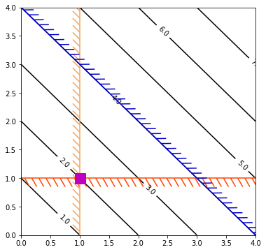
2d example with matplotlib

x1, x2 = sy.symbols(['x1', 'x2'], positive=True)
syms = [x1, x2]
f = Function(x1 + x2, variables=syms)
ieq1 = InEquality(x1 - 1, op='>=', variables=syms)
ieq2 = InEquality(x2 - 1, op='>=', variables=syms)
ieq3 = InEquality(x1 + x2 - 4, op='<=', variables=syms)
lpp = LPP(cost=f, constraints=[ieq1, ieq2, ieq3], variables=syms)
x = atleast2d(lpp.solve()['x'])

import numpy as np
import matplotlib.pyplot as plt
from matplotlib import patheffects

fig, ax = plt.subplots(figsize=(6, 6))

nx = 101
ny = 105

# Set up survey vectors
xvec = np.linspace(0.001, 4.0, nx)
yvec = np.linspace(0.001, 4.0, ny)

# Set up survey matrices.  Design disk loading and gear ratio.
x1, x2 = np.meshgrid(xvec, yvec)

# Evaluate some stuff to plot
obj = x1 + x2
g1 = x1 - 1
g2 = x2 - 1
g3 = x1 + x2 - 4

cntr = ax.contour(x1, x2, obj, colors='black')
ax.clabel(cntr, fmt="%2.1f", use_clabeltext=True)

cg1 = ax.contour(x1, x2, g1, [0], colors='sandybrown')
plt.setp(cg1.collections, path_effects=[
         patheffects.withTickedStroke(angle=-135)])

cg2 = ax.contour(x1, x2, g2, [0], colors='orangered')
plt.setp(cg2.collections, path_effects=[
         patheffects.withTickedStroke(angle=-60)])

cg3 = ax.contour(x1, x2, g3, [0], colors='mediumblue')
plt.setp(cg3.collections, path_effects=[patheffects.withTickedStroke()])

ax.plot(x[:, 0], x[:, 1], 'ms', markersize=15)

ax.set_xlim(0, 4)
ax.set_ylim(0, 4)

plt.show()

Solution with a Binary Genetic Algorithm (BGA)

It’s completely nuts to solve LLPs with a GA, but wrapping up an LLP in standard form is actually quite easy and makes for a good example.

x1, x2 = sy.symbols(['x1', 'x2'], positive=True)
syms = [x1, x2]
f = Function(x1 + x2, variables=syms)
ieq1 = InEquality(x1 - 1, op='>=', variables=syms)
ieq2 = InEquality(x2 - 1, op='>=', variables=syms)
ieq3 = InEquality(x1 + x2 - 4, op='<=', variables=syms)
lpp = LPP(cost=f, constraints=[ieq1, ieq2, ieq3], variables=syms)
lpp.solve()['x']

array([1., 1.])

The BGA imlmeneted in dewloosh.math.optimize does not accept constraints, all the requirements must be cooked into the objective function. A simple way of accomplishing this is to add penalties to the objective on constraint violations:

def cost(x):
    return lpp.obj(x) if lpp.feasible(x) else lpp.obj(x) + 1e12

BinaryGeneticAlgorithm(cost, [[0, 4], [0, 4]], length=12, nPop=200).solve()

array([1.0002442, 1.0002442])